Kuramoto network optimization

gradnet concepts demonstrated below

ODE integration via gradnet.integrate_ode

A loss function for a dynamical system

Optimizer selection

Logging using TensorBoard

Checkpointing

Animation

Problem setup

Consider the Kuramoto model for nodes with internal frequencies \(\{\omega_i\}_{i=1}^N\) with weighted adjacency matrix \(A_{ij}\) obaying the dynamics:

\[ \frac{d\theta_i}{dt} = \omega_i + \sum_{j=1}^N A_{ij} \sin(\theta_j - \theta_i) \]

Notice, that the adjacency matrix here is weighted: \(A_{ij}=0\) if there is no edge between nodes \(i\) and \(j\), otherwise \(A_{ij}\) is the edge-weight of the existing edge.

For this model, we seek the optimal network, with the fixed total edge-weight budget which supports the strongest synchronization.

Synchronization in Kuramoto model is measured as:

\[ r(t) = \left| \frac{1}{N} \sum_{j=1}^N e^{i\theta_j(t)} \right| \]

where \(r(t) \in [0, 1]\) measures the degree of phase synchronization at time \(t\). This is implemented in the function loss_fn.

Vectorizing the ODE (Optional)

We can simplify the right-hand-side of the ODE by applying the trig identity \(\sin(a-b) = \cos(a)\sin(b) - \sin(a)\cos(b)\), which allows efficient vectorized computation of the interaction term. The resulting vectorized ODE is:

\[ \frac{d\boldsymbol{\theta}}{dt} = \boldsymbol{\omega} + \left[ \cos(\boldsymbol{\theta}) \odot (A\cdot \sin(\boldsymbol{\theta})) - \sin(\boldsymbol{\theta}) \odot (A\cdot \cos(\boldsymbol{\theta})) \right] \]

where \(\odot\) denotes the Hadamard (element-wise) product. This is implemented in the function dθ_dt in the code

Note: vectorization is not required, but it helps accelerate the computations (especially if using a GPU).

Install

install the required dependencies silently

%%capture
!pip install 'gradnet[examples]'

GradNet optimization

from gradnet import GradNet, integrate_ode, fit
from gradnet.utils import plot_adjacency_heatmap, plot_graph
import numpy as np
import torch
import matplotlib.pyplot as plt
from matplotlib.cm import bwr


# set up problem parameters preferably in Torch
N = 100
budget_per_node = 2.0
ω = np.linspace(0, 1, N)  # uniformly distributed natural frequencies in [0, 1]
ω = torch.tensor(ω)  # convert to torch tensor

gn = GradNet(num_nodes=N, budget=budget_per_node*N, rand_init_weights=False, 
             delta_sign="nonnegative", final_sign="free", strict_budget=True)  # create the GradNet instance

def dθ_dt(t, θ, A, ω):
    # Kuramoto model: dθ_i/dt = ω_i + Σ A_ij sin(θ_j - θ_i)
    sinx = torch.sin(θ)
    cosx = torch.cos(θ)
    return ω + cosx * (A @ sinx) - sinx * (A @ cosx)

def loss_fn(gn):
    tt = torch.linspace(0, 5, 150)  # time grid to evaluate the numerical solutions
    θ0 = torch.zeros(N)  # set the initial phases to 0 (this choice accelerates traning)

    f_params = {"ω": ω}  # contains every parameter of the dθ_dt beyond t, θ, and A. 
    tt, θθ = integrate_ode(gn, f=dθ_dt, x0=θ0, tt=tt, f_kwargs=f_params)  # integrate the ODE

    rr = torch.abs(torch.mean(torch.exp(1j * θθ), dim=1)) # compute the synchronization time series
    r_mean = torch.mean(rr)  # average it over time

    return 1 - r_mean, {'r':r_mean}  # loss function is minimized, so in order to maximize synch, 


fit(gn=gn, 
    loss_fn=loss_fn, 
    num_updates=600, 
    optim_cls=torch.optim.Adam, optim_kwargs={"lr": 1, "betas": (0.9, 0.999)}, 
    accelerator="cpu",
    logger=True,
    enable_checkpointing=True, checkpoint_dir="./kuramoto_checkpoints", checkpoint_every_n=1);

loss, measures = loss_fn(gn)
print(f"optimal synchrony: {measures['r']}")

fig, (ax0, ax1) = plt.subplots(1, 2, figsize=(10, 4), constrained_layout=True)
plot_adjacency_heatmap(gn, ax=ax0)
plot_graph(gn, ax=ax1, draw_kwargs={'node_color': ω, 'cmap': bwr}, colorbar_label="ω")

GPU available: True (mps), used: False
TPU available: False, using: 0 TPU cores
HPU available: False, using: 0 HPUs

  | Name | Type    | Params | Mode 
-----------------------------------------
0 | gn   | GradNet | 10.0 K | train
-----------------------------------------
10.0 K    Trainable params
0         Non-trainable params
10.0 K    Total params
0.040     Total estimated model params size (MB)
`Trainer.fit` stopped: `max_epochs=600` reached.

optimal synchrony: 0.9985901117324829

<networkx.classes.graph.Graph at 0x323ad7750>

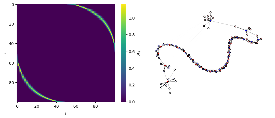
../_images/6056f7f58bae75a2597ebd139f3c69a31c5cec77df64d1fec2bde473e34844b0.png

On the left, the optimized adjacency matrix is plotted as a heatmap.

On the right, we show the sppring layout plot of the resulting weighted network. The edgeweights are repreented as the edge widths, and the node colors correspond to their intrinsic frequencies.

Let’s animate the adjacency matrix from the checkpoints

from gradnet.utils import animate_adjacency

animate_adjacency("./kuramoto_checkpoints");

TensorBoard

To track live plots of loss and other scalars (like the number of missclassified edges in this case), you first need to ensure that tensorboard is installed: type pip install tensorboard in terminal. Then you should navigate your a terminal to your python project directory and type: tensorboard --logdir .