Spectral optimization (algebraic connectivity)
Main
gradnetconcepts demonstrated below
Configuring a
GradNetmodel for network optimizationDefining a loss function
Training the network structure using
fitAccelerator selection (cpu/gpu)
Learning rate selection
Extracting and visualizing the optimized networks
Converting to NetworkX
Using a mask to ignore forbidden edges (e.g., grid)
Problem setup
The second Laplacian eigenvalue, also known as the algebraic connectivity of the network, is a quantitative measure of connectivity and robustness. It indicates how “tightly held together” a network is, governs how fast diffusion converges on it, and reveals natural partitions in its structure. We ask how to allocate finite edgeweight resources (the budget) on a 2D grid in order to maximize the algebraic connectivity.
Install
install the required dependencies silently
%%capture
!pip install 'gradnet[examples]'
GradNet optimization
from gradnet import GradNet, fit
from gradnet.utils import plot_adjacency_heatmap, plot_graph, random_seed, to_networkx
import torch
from matplotlib import pyplot as plt
import tensorboard
import numpy as np
import networkx as nx
import cmcrameri.cm as cmc

random_seed(42)

# define the loss function
def loss_fn(gn):
    A = gn()  # get the adjacency matrix?
    L = torch.diag(A.sum(dim=1)) - A  # compute the graph Laplacian
    eigs = torch.linalg.eigvalsh(L)  # compute the eigenvalues
    l2 = eigs[1]  # second smallest eigenvalue (algebraic connectivity)
    # loss is (1-λ₂), so minimizing it maximizes λ₂.
    return 1-l2, {"λ₂": l2, "λ_3": eigs[2], "λ_4": eigs[3]}  # return loss, and also λ₂ as a metric

rows = 30
cols = 30
budget_per_node = 1

N = rows * cols

def make_grid_mask(rows, cols):
    mask_nx = nx.grid_2d_graph(rows, cols)  # Build grid graph (nodes are (r, c) tuples)
    nodes = sorted(mask_nx.nodes())  # sort nodes
    return nx.to_numpy_array(mask_nx, nodelist=nodes)

mask = make_grid_mask(rows, cols)

gn_grid = GradNet(num_nodes=N, budget=budget_per_node * N, mask=mask, rand_init_weights=0)
lightning_trainer, best_ckpt = fit(gn=gn_grid, loss_fn=loss_fn, num_updates=300, optim_kwargs={"lr": 0.001}, accelerator="cpu")
GPU available: True (mps), used: False
TPU available: False, using: 0 TPU cores
HPU available: False, using: 0 HPUs
  | Name | Type    | Params | Mode
-----------------------------------------
0 | gn   | GradNet | 810 K  | train
-----------------------------------------
810 K     Trainable params
0         Non-trainable params
810 K     Total params
3.240     Total estimated model params size (MB)
`Trainer.fit` stopped: `max_epochs=300` reached.
Plot the result as a grid
net = to_networkx(gn_grid)
pos = {r * cols + c: (c, -r) for r in range(rows) for c in range(cols)}

edge_w = np.fromiter(nx.get_edge_attributes(net, "weight").values(), dtype=float)

fig, ax = plt.subplots(figsize=(3, 2.), dpi=300)
nx.draw_networkx_edges(net, pos, ax=ax, edge_color=edge_w, edge_cmap=cmc.managua, width=1.5)
nx.draw_networkx_nodes(net, pos, ax=ax, node_color="k", node_size=1.6)
ax.set_axis_off()

sm = plt.cm.ScalarMappable(cmap=cmc.managua)
sm.set_array(edge_w)
fig.colorbar(sm, ax=ax, label="edge weight")

plt.tight_layout()
plt.show()
/var/folders/72/79vqt54j447byqmvb80g_n3w0000gn/T/ipykernel_97545/3945664359.py:7: DeprecationWarning: `alltrue` is deprecated as of NumPy 1.25.0, and will be removed in NumPy 2.0. Please use `all` instead.
  nx.draw_networkx_edges(net, pos, ax=ax, edge_color=edge_w, edge_cmap=cmc.managua, width=1.5)
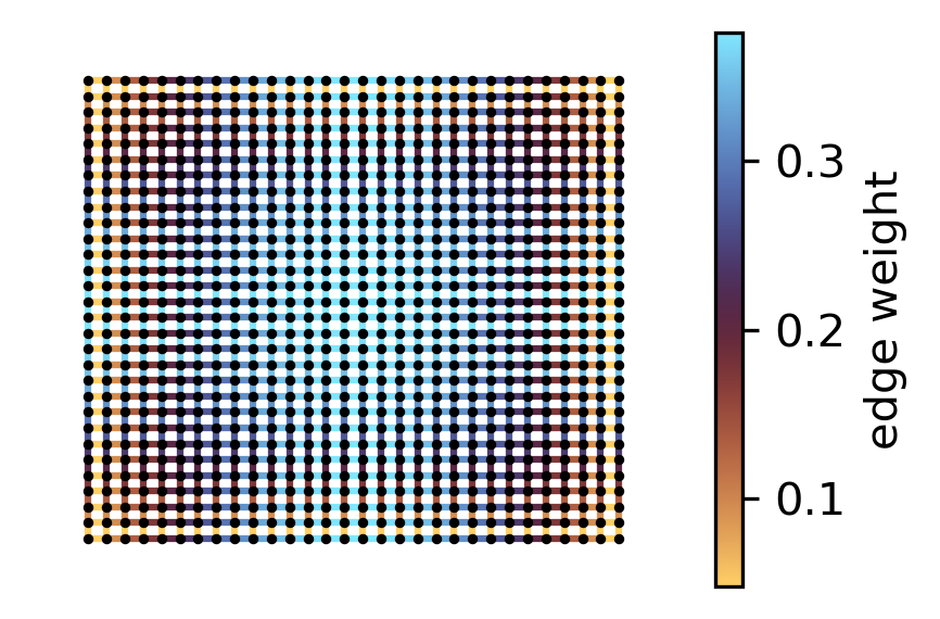
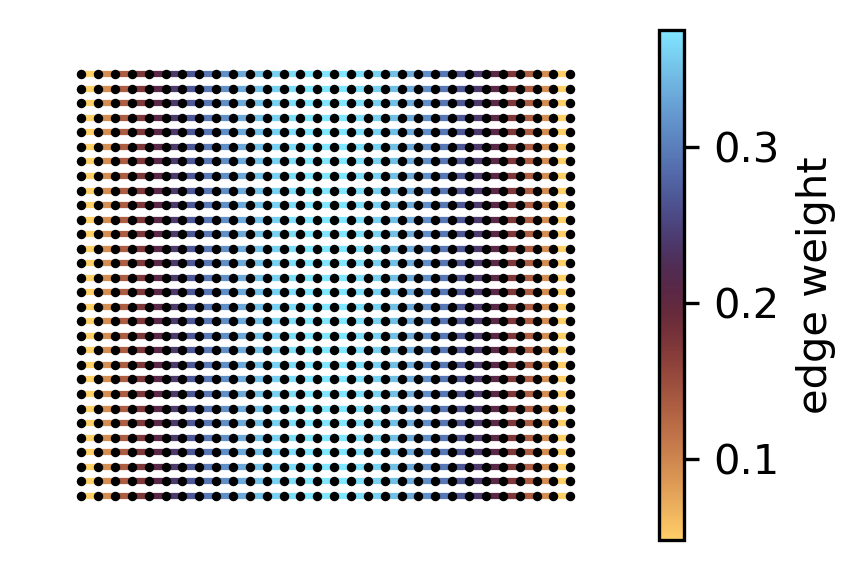
This indicates that, on a grid, edges near the center play a critical role and should be prioritized with more resources to enhance Algebraic Connectivity. In fact, the optimal weights of horizontal edges depends exclusively on their horizontal position in the grid, and vertical edge weights only depend on their vertical position.
Now plot horizontal edges only
# horizontal edges only (same row -> same y in pos)
h_edges = [(u, v) for (u, v) in net.edges() if pos[u][1] == pos[v][1]]
h_w = np.array([net[u][v].get("weight", np.nan) for (u, v) in h_edges], dtype=float)

# fig, ax = plt.subplots(figsize=(6, 4.5))
# nx.draw_networkx_edges(net, pos, ax=ax, edgelist=h_edges, edge_color=h_w, edge_cmap=cmc.managua, width=3)
# nx.draw_networkx_nodes(net, pos, ax=ax, node_color="k", node_size=3)
fig, ax = plt.subplots(figsize=(3, 2.), dpi=300)
nx.draw_networkx_edges(net, pos, ax=ax, edgelist=h_edges, edge_color=h_w, edge_cmap=cmc.managua, width=1.5)
nx.draw_networkx_nodes(net, pos, ax=ax, node_color="k", node_size=1.6)

ax.set_axis_off()

sm = plt.cm.ScalarMappable(cmap=cmc.managua)
sm.set_array(h_w)
fig.colorbar(sm, ax=ax, label="edge weight")

plt.tight_layout()
plt.show()
/var/folders/72/79vqt54j447byqmvb80g_n3w0000gn/T/ipykernel_97545/3821016335.py:9: DeprecationWarning: `alltrue` is deprecated as of NumPy 1.25.0, and will be removed in NumPy 2.0. Please use `all` instead.
  nx.draw_networkx_edges(net, pos, ax=ax, edgelist=h_edges, edge_color=h_w, edge_cmap=cmc.managua, width=1.5)
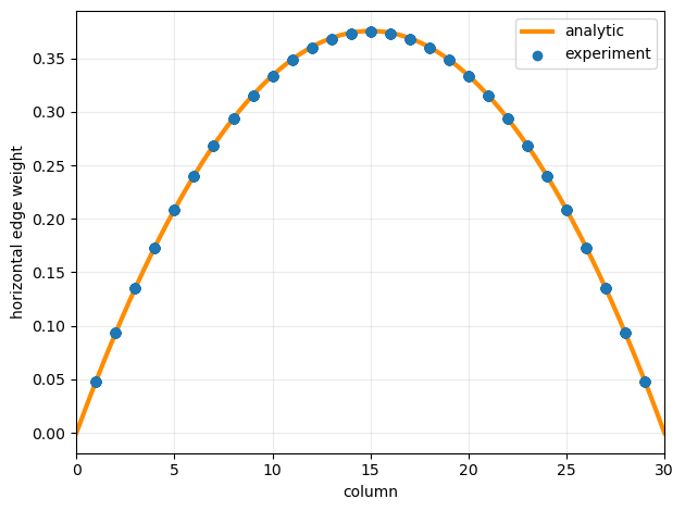
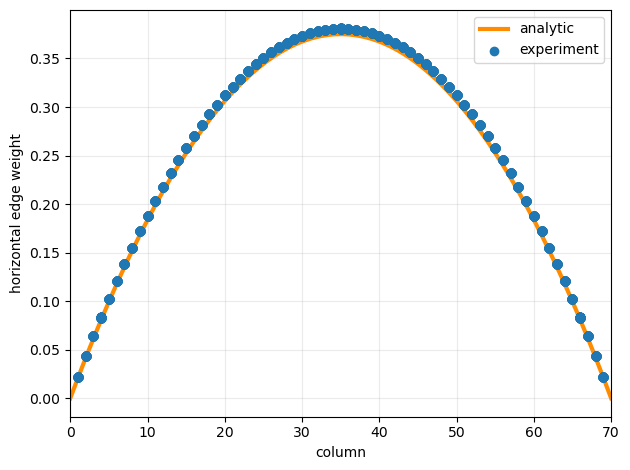
Comparing optimal edge-weights to the analytical expectation (reference will be added soon)
def plot_horizontal_edgeweights(net):
    # Horizontal edges + their 1-based column location
    edges_h = [(u, v) for (u, v) in net.edges()
            if (u // cols == v // cols) and (abs(u - v) == 1)]

    xh_col = [min(u % cols, v % cols) + 1 for (u, v) in edges_h]   # 1..cols-1
    wh     = [net[u][v]["weight"] for (u, v) in edges_h]

    xx = np.linspace(0, cols, 400)
    yy = (3/2) * budget_per_node / ((rows - 1) * (rows + 1)) * xx * (rows - xx)

    plt.figure()
    plt.plot(xx, yy, label="analytic", zorder=1, linewidth=3, color="darkorange")
    plt.scatter(xh_col, wh, zorder=2, label="experiment")

    plt.xlabel("column")
    plt.ylabel("horizontal edge weight")
    plt.xlim(0, cols)
    plt.grid(True, alpha=0.25)
    plt.legend()
    plt.tight_layout()
    plt.show()

plot_horizontal_edgeweights(net)
Sparse vs dense encodings
Below we implement the same optimization task with sparse GradNet representation. Gradnet uses it’s sparse backend whenever a sparse torch tensor is provided as a mask. Yet, torch.linalg.eigvalsh expects a dense matrix, but densifying the GradNet output is counterproductive. So we define the sparse alternative relying on the power method. For detailed theory see [1].
# power method for finding λ₂ (avoids dense matrix operations)
def sparse_loss(gn, n_iter=10000, eps=0.):
    A = gn()  # sparse adjacency
    n = A.size(0)

    ones = torch.ones(n, 1, device=A.device, dtype=A.dtype)
    d = torch.sparse.mm(A, ones).squeeze(1)
    d_max = d.max().detach()
    c = 2.0 * d_max + eps

    with torch.no_grad():
        # random_seed(0)
        x = torch.randn(n, 1, device=A.device, dtype=A.dtype)
        x = x - x.mean()
        x = x / x.norm()

        for _ in range(n_iter):
            Ax = torch.sparse.mm(A, x)
            Lx = d.unsqueeze(1) * x - Ax
            y = c * x - Lx
            y = y - y.mean()
            x = y / y.norm()

    Ax = torch.sparse.mm(A, x)
    Lx = d.unsqueeze(1) * x - Ax
    lambda2 = (x.t() @ Lx) / (x.t() @ x)
    lambda2 = lambda2.squeeze()

    loss = 1.0 - lambda2
    return loss, {"λ₂": lambda2, "c": c}

def make_sparse_grid_mask(rows, cols, device=None, dtype=None):
    n = rows * cols
    device = device or "cpu"
    dtype = dtype or torch.get_default_dtype()
    if n == 0:
        return torch.sparse_coo_tensor(torch.empty((2,0),dtype=torch.long,device=device),
                                       torch.empty((0,),dtype=dtype,device=device),
                                       (0,0)).coalesce()
    ids = torch.arange(n, device=device).view(rows, cols)
    a,b = ids[:, :-1].ravel(), ids[:, 1:].ravel()
    c,d = ids[:-1, :].ravel(), ids[1:, :].ravel()
    src = torch.cat([a,b,c,d]); dst = torch.cat([b,a,d,c])
    return torch.sparse_coo_tensor(torch.stack([src,dst]),
                                   torch.ones(src.numel(), device=device, dtype=dtype),
                                   (n,n)).coalesce()
Let us let us optimize 70*70=4900 node grid
rows = 70
cols = 70
budget_per_node = 1

N = rows * cols

mask = make_sparse_grid_mask(rows, cols, device="cpu")  # generate a sparse mask


gn_sparse = GradNet(num_nodes=N, budget=budget_per_node * N, mask=mask, rand_init_weights=False)

sparse_accurate_loss = lambda x: sparse_loss(x, n_iter=50000)

lightning_trainer, best_ckpt = fit(gn=gn_sparse,
                                   loss_fn=sparse_accurate_loss,
                                   num_updates=100,
                                   optim_kwargs={"lr": 0.01},
                                   accelerator="cpu");
GPU available: True (mps), used: False
TPU available: False, using: 0 TPU cores
HPU available: False, using: 0 HPUs
  | Name | Type    | Params | Mode
-----------------------------------------
0 | gn   | GradNet | 9.7 K  | train
-----------------------------------------
9.7 K     Trainable params
0         Non-trainable params
9.7 K     Total params
0.039     Total estimated model params size (MB)
`Trainer.fit` stopped: `max_epochs=100` reached.
Plot the result
net = to_networkx(gn_sparse)
plot_horizontal_edgeweights(net)
Now let us run this optimization for various sized systems and observe how computation time scales. In order to accelerate the computations, we will perform just 5 iterations. The plots will be for more realistic 50 iterations. You can skip this cell to save time, next cell has the data in a list format already.
import time

ll = 10 + 5 * np.arange(20)
times_s = np.array([])
times_d = np.array([])
for l in ll:
    for dense in [0, 1]:

        rows = l
        cols = l
        budget_per_node = 1

        N = rows * cols

        mask = make_sparse_grid_mask(rows, cols)
        if dense:
            mask = mask.to_dense()

        gn_sparse = GradNet(num_nodes=N, budget=budget_per_node * N, mask=mask, rand_init_weights=False)

        t0 = time.perf_counter()
        lightning_trainer, best_ckpt = fit(gn=gn_sparse, loss_fn=sparse_loss, num_updates=5, optim_kwargs={"lr": 0.05}, accelerator="cpu", verbose=False);
        if dense:
            times_d = np.append(times_d, time.perf_counter() - t0)
        else:
            times_s = np.append(times_s, time.perf_counter() - t0)
        print(f"l={l}, {'dense' if dense else 'sparse'}, time= {time.perf_counter() - t0:.5f} s")
l=10, sparse, time= 0.95737 s
l=10, dense, time= 0.85152 s
l=15, sparse, time= 1.14507 s
l=15, dense, time= 1.21797 s
l=20, sparse, time= 1.49741 s
l=20, dense, time= 1.20950 s
l=25, sparse, time= 1.93709 s
l=25, dense, time= 1.68341 s
l=30, sparse, time= 2.58147 s
l=30, dense, time= 2.40908 s
l=35, sparse, time= 3.44847 s
l=35, dense, time= 3.34129 s
l=40, sparse, time= 4.04532 s
l=40, dense, time= 3.72016 s
l=45, sparse, time= 5.04807 s
l=45, dense, time= 7.40627 s
l=50, sparse, time= 5.82292 s
l=50, dense, time= 17.26017 s
l=55, sparse, time= 6.83997 s
l=55, dense, time= 32.59824 s
l=60, sparse, time= 8.04761 s
l=60, dense, time= 53.41051 s
l=65, sparse, time= 9.38997 s
l=65, dense, time= 74.64365 s
l=70, sparse, time= 10.58996 s
l=70, dense, time= 106.27724 s
l=75, sparse, time= 12.21190 s
l=75, dense, time= 135.10198 s
l=80, sparse, time= 13.78168 s
l=80, dense, time= 161.77623 s
l=85, sparse, time= 15.48220 s
l=85, dense, time= 232.14943 s
l=90, sparse, time= 17.28782 s
l=90, dense, time= 299.51368 s
l=95, sparse, time= 20.40560 s
l=95, dense, time= 358.98417 s
l=100, sparse, time= 21.30333 s
l=100, dense, time= 438.99194 s
l=105, sparse, time= 23.56510 s
l=105, dense, time= 518.49347 s
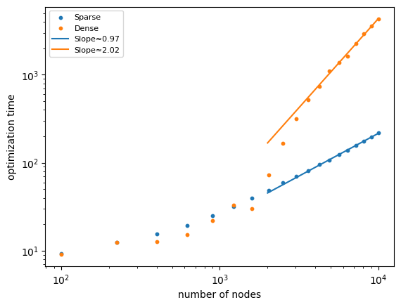
Finally we will plot the scaling of computation time vs sparse and dense encoded network sizes. Measurements from the previous cell are stored as two np lists in the next cell: sparse and dense
import numpy as np
import matplotlib.pyplot as plt

# Data
ll = 10 + 5 * np.arange(19)
n = ll**2

sparse = 10*np.array([
    0.93218, 1.24371, 1.55464, 1.94781, 2.51872, 3.20490, 3.94379, 4.84548, 5.92074, 6.96476,
    8.15329, 9.53883, 10.73403, 12.44468, 13.79658, 15.65240, 17.47435, 19.76382, 21.89966
])

dense = 10*np.array([
    0.90607, 1.25043, 1.25943, 1.52722, 2.21107, 3.30257, 3.02127, 7.23395, 16.54406, 31.43409,
    51.56717, 74.36497, 110.18030, 136.74495, 163.21513, 227.38628, 294.51242, 358.31103, 431.86417
])

# Fit power laws using the last 8 points
fit_last = 8
n_fit = n[-fit_last:]
sparse_fit = sparse[-fit_last:]
dense_fit = dense[-fit_last:]

log_n = np.log(n_fit)
log_sparse = np.log(sparse_fit)
log_dense = np.log(dense_fit)

slope_sparse, intercept_sparse = np.polyfit(log_n, log_sparse, 1)
slope_dense, intercept_dense = np.polyfit(log_n, log_dense, 1)

# Extend fit lines
n_line = np.linspace(2000, 10000, 400)
sparse_line = np.exp(intercept_sparse) * n_line**slope_sparse
dense_line = np.exp(intercept_dense) * n_line**slope_dense

# Plot
plt.figure()

plt.scatter(n, sparse, label="Sparse", s=10)
plt.scatter(n, dense, label="Dense", s=10)

plt.loglog(n_line, sparse_line,
           label=f"Slope≈{slope_sparse:.2f}")

plt.loglog(n_line, dense_line,
           label=f"Slope≈{slope_dense:.2f}")

plt.xscale("log")
plt.yscale("log")

plt.xlabel("number of nodes")
plt.ylabel("optimization time")

plt.legend(fontsize=8)
plt.show()